Today, users have high expectations for the programs they use. Users expect programs to have amazing features, to be fast, and to consume a reasonable amount of memory.

As developers, we should thrive to give our users the best experience possible. We need to find and eliminate the bottlenecks before they affect our users. Unfortunately, as programs become more and more complex, it becomes harder to find those issues and bottlenecks.

Today, I am going to focus on a technique to find those bottlenecks, and this technique is profiling. My goal today is to show you that profiling is not rocket science. Everyone can find their bottlenecks without breaking a sweat.

The code for this article can be found on GitHub, and a more detailed recorded version can be found on YouTube.

‍

Profiling Definition and Benefits

A profile is a set of statistics that describes how our program is executed. When we know how different parts of our code behave, we can use this information to optimize our code.

You must be asking yourself why should I even care about optimizing my code, my feature is already done. You should care about optimization because it affects our users and our company. These are the main reasons:

Fast programs are better than slow ones — whether latency or throughput.
Memory efficiency is good — Most of us are terrified of out-of-memory errors.
Saving money is awesome — If out-of-memory errors do not terrify you, your AWS bills might.
Hardware has limits— Even if we are willing to pay to improve performance, hardware will only take you so far.

Hopefully I have convinced you that profiling is a concept that every programmer needs in his toolbox. But before we jump into the water, I am going to cover some safety rules.

‍

Safety Rules

The following rules were written with blood.

Make sure it’s actually needed — Optimized code tends to be harder to write and read, which makes it less maintainable and buggier. We need to gather the requirements (SLA/SLOS) to understand our definition of “done.”
Make sure our code is well tested — I know everyone says it, but it's really important. It will be sad if we fix the performance problem, but our program will not work.
Good work takes cycles — We should focus on the problematic parts of the code (the bottleneck).

Now we’ve gone through the safety rules, we can finally jump into the water and get to know what types of profilers exist.

‍

Types of Profilers

When we want to find our bottleneck, we need to use the right tool for the job, as there is no free lunch.

Picking the right tool for the job depends on the following characteristics:

The resource we want to measure — whether it's CPU, RAM, I/O, or other exotic metrics.
Profiling strategy — how the profiler collects the data: in a deterministic manner using hooks or in a statistical manner by collecting information at each time interval.
Profiling granularity — at what level we get the information: program level, function level, or line level. Obviously, we can extract more insights if we use finer granularity levels, like line level, but that will add a lot of noise.

‍

Our Example

In this article, I am going to use Peter Norvig’s naive spelling corrector. Norvig’s spelling corrector uses the Levenshtein distance to find spelling mistakes.

“The Levenshtein distance is a string metric for measuring the difference between the two words. The distance between two words is the minimum number of single-character edits (i.e., insertions, deletions, or substitutions) required to change one word into the other.” — The Levenshtein Distance Algorithm

Norvig’s spelling corrector corrects spelling mistakes by finding the most probable words with a Levenshtein distance of two or less. This spelling corrector seems quite naive, but it actually achieves 80% or 90% accuracy.


import re
from collections import Counter

def words(text): 
    return re.findall(r'\w+', text.lower())

WORDS = Counter(words(open('big.txt').read()))

def P(word, N=sum(WORDS.values())): 
    return WORDS[word] / N

def candidates(word): 
    return (known([word]) or known(edits1(word)) or known(edits2(word)) or [word])

def known(words): 
    return set(w for w in words if w in WORDS)

def edits1(word):
    letters    = 'abcdefghijklmnopqrstuvwxyz'
    splits     = [(word[:i], word[i:])    for i in range(len(word) + 1)]
    deletes    = [L + R[1:]               for L, R in splits if R]
    transposes = [L + R[1] + R[0] + R[2:] for L, R in splits if len(R)>1]
    replaces   = [L + c + R[1:]           for L, R in splits if R for c in letters]
    inserts    = [L + c + R               for L, R in splits for c in letters]
    return set(deletes + transposes + replaces + inserts)

def edits2(word): 
    return (e2 for e1 in edits1(word) for e2 in edits1(e1))

def word_correction(word): 
    return max(candidates(word), key=P)

def sentence_correction(sentence): 
    return " ".join(word_correction(word) for word in sentence.split(" "))

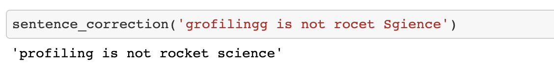
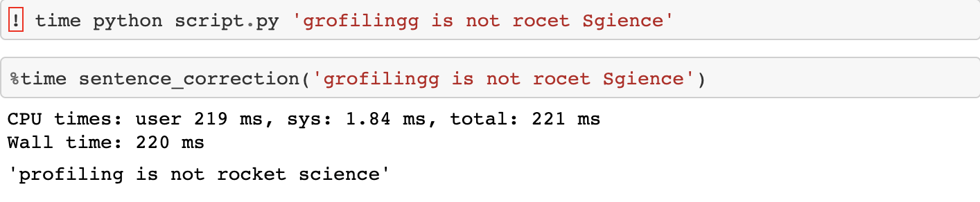
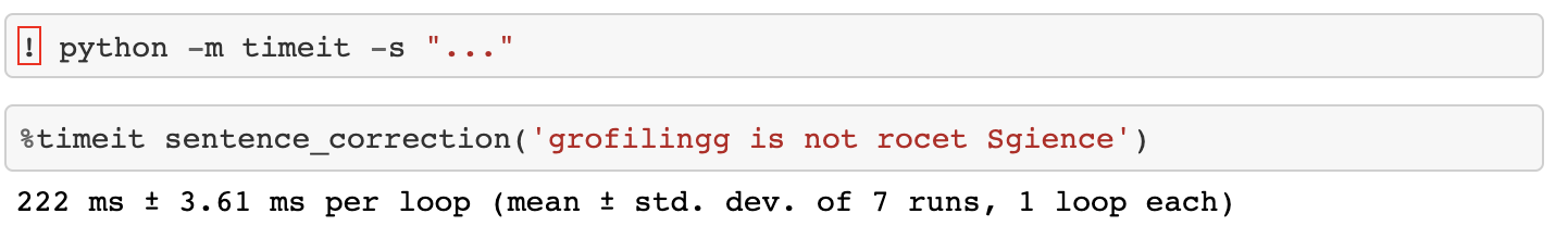
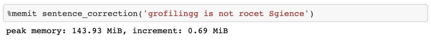
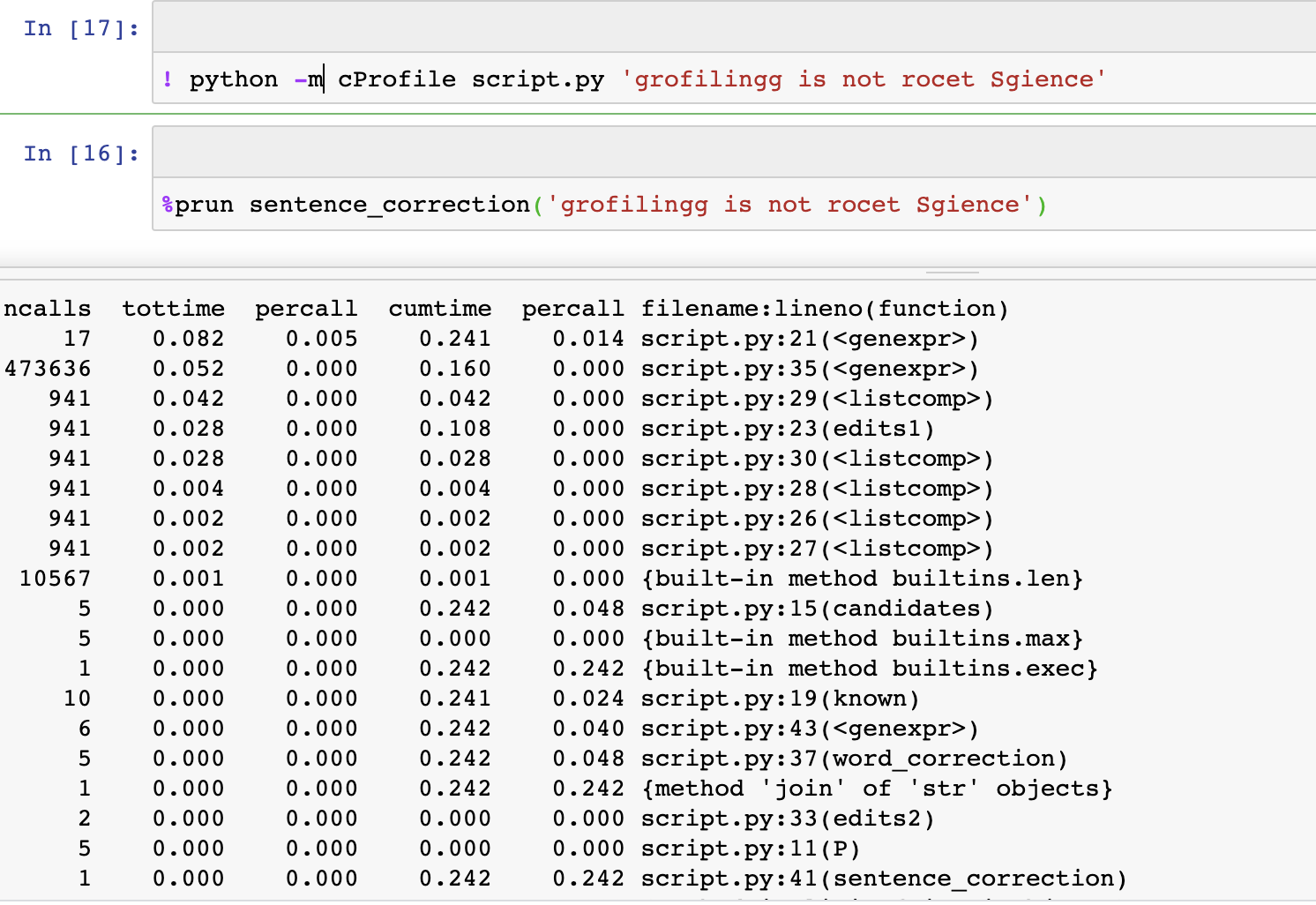
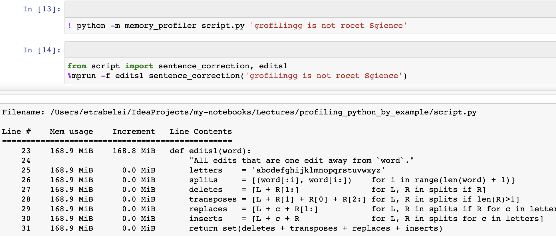
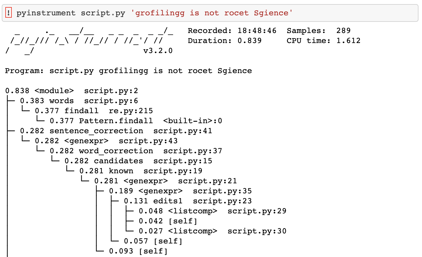
We can use our spelling corrector to understand the following message “grofilingg is not rocet Sgience,” and we get “profiling is not rocket science.”

Norvig’s spelling corrector showing a sentence full of spelling errors corrected to “profiling is not rocket science”

We will start profiling our example with the first type of profiler, casual profilers.

‍

Casual Profilers

Casual profilers give us a sense of how the program runs as a whole and allow us to understand whether a problem exists.

The first tool we going to cover is time, which helps us measure the user and system time for a single run. It is built-in in Python and comes with IPython magic, no additional installation is required.

The Wall time is the overall execution time, and the CPU time is the time that the program uses the CPU. In our example, we can see the Wall time is 220 milliseconds and 219 of it is spent on CPU, which means we are CPU bound.

‍

The next tool I am going to cover is the timeit module, which helps us measure the execution time of multiple runs. It is built-in in Python, and comes with IPython, no additional installation required. It uses some neat tricks, like disabling the garbage collection, to make the result more consistent.

Norvig’s spelling corrector showing the performance times for a spelling correction — We can see that it was executed our program 7 times and the average execution time is 22 milliseconds with a 3.6 milliseconds variation between the executions.

‍

The last tool for casual profiling I am going to cover today is memit magic, which helps us measure the process memory. It not built-in in Python, so installation is required, but after we install it, we can use IPython magic.

‍

Norvig’s spelling corrector showing memory performance for a spelling correction — The peak memory is the largest memory used by the process, and the increment is how much this specific call added to memory consumption. We can see that correcting one sentence increases memory consumption in 0.69 Mib.

‍

There are a few more casual profiling tools, and the casual profiling landscape ️️️️looks as follows:

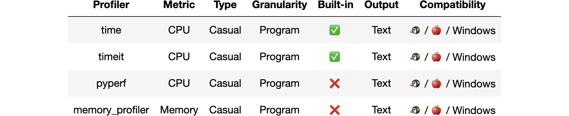
table comparing several casual profiling tools — The casual profiling landscape ️️️️

‍

Casual profilers have the following pros and cons

They are really easy to use.
They allow us to understand whether a problem exists.
But we can’t use them to pinpoint the bottleneck.

The fact that we can’t pinpoint the bottleneck is crucial and leads us to the next set of profilers, offline profilers.

‍

Offline Profilers

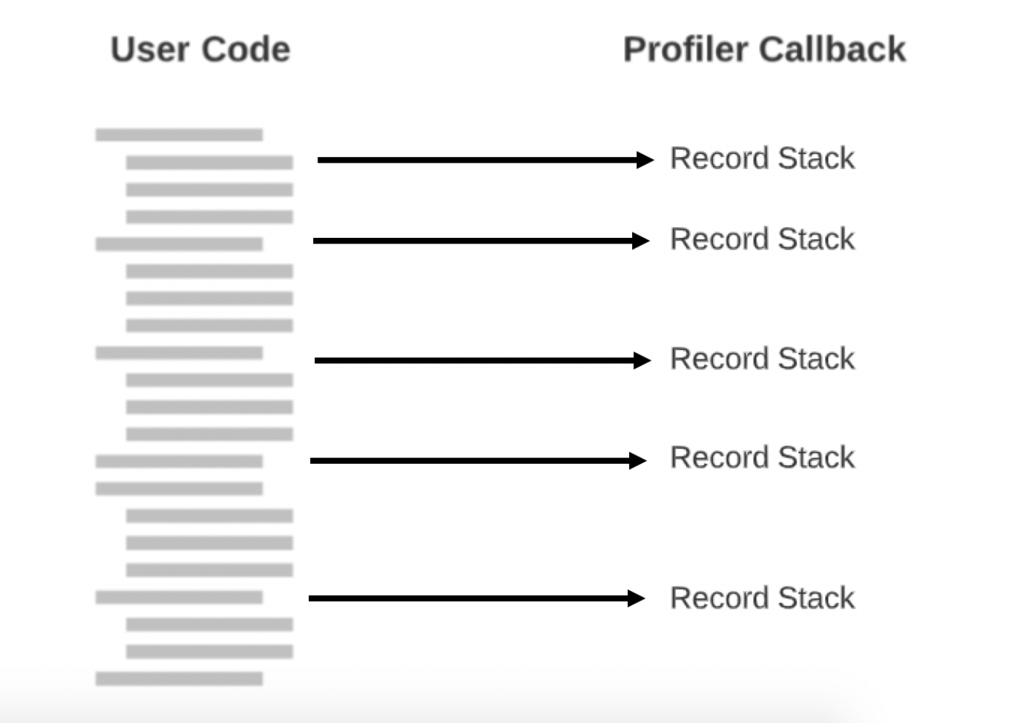
Offline profilers help us to understand the behavior of our program by tracking events like function calls, exceptions, and line executions. Because they execute hooks on specific events, they are deterministic and add significant overhead, which makes them more suitable for local debugging.

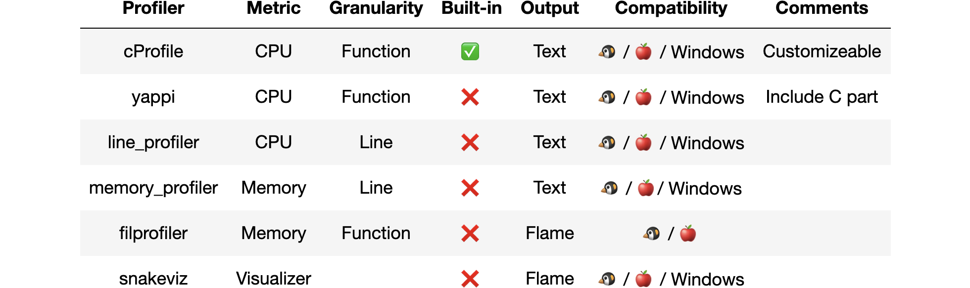
a diagram illustrating how a callback records the stack — Python lets you specify a callback on specific interpreter events using *sys.setprofile* or sys.settrace. The callback records the stack.

The first tool we going to cover is the cProfile, which traces every function call and allows us to identify time-consuming functions. By default, it measures the process CPU but allows us to specify our own measurement. It is built-in in Python and comes with IPython magic, no additional installation is required. cProfile works only on the Python level and doesn’t work across multiple processes.

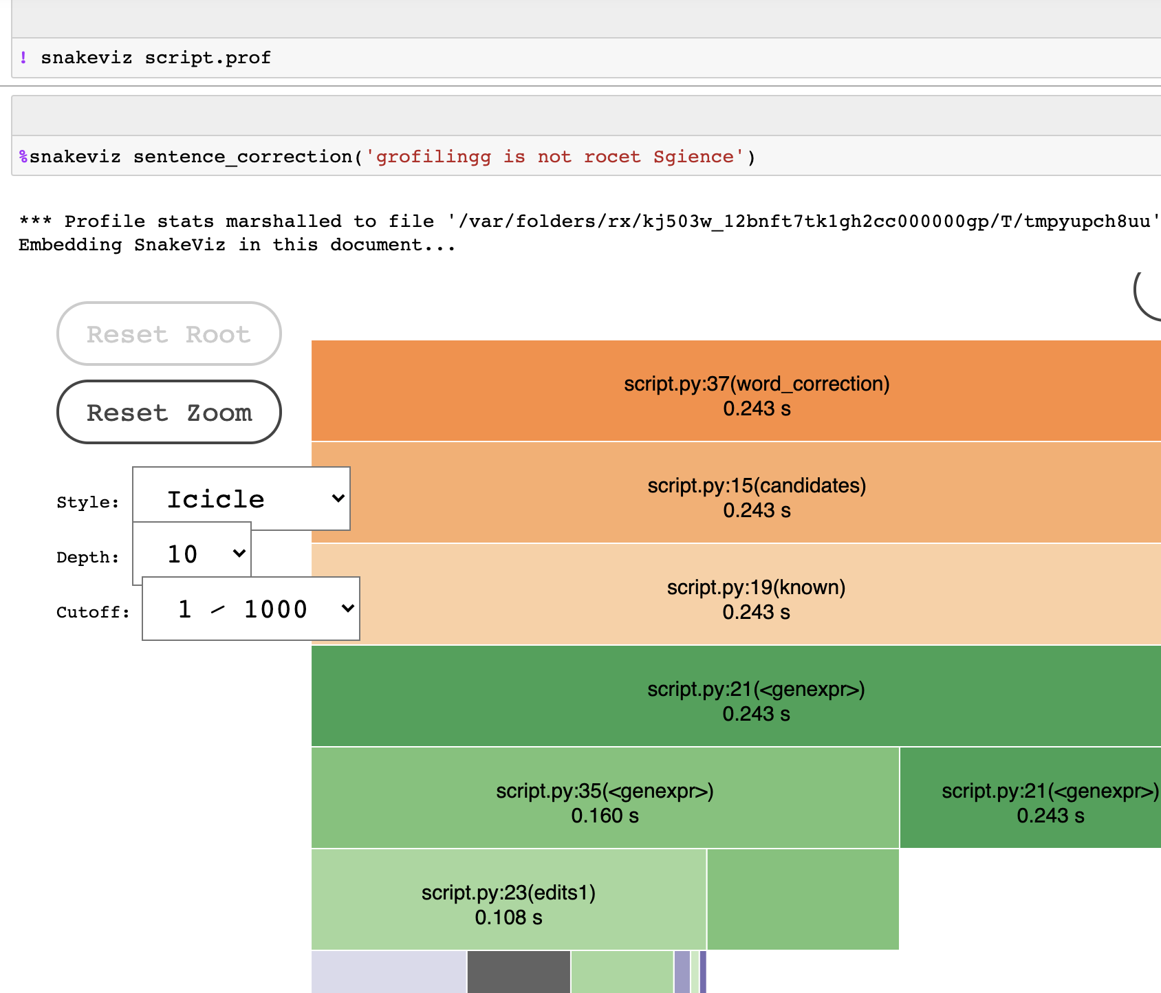
a table of performance statistics for the sentence_correction function of cProfile — We can see our sentence_correction function took 0.24 seconds. All of it spent on the candidate function, and when we drill down, the edits1 takes 0.1 seconds (40%).

It’s a lot of text to handle, and a bit encrypted for first comers. For this reason, the next tool was invented, SnakeViz. SnakeViz takes cProfile output and creates intuitive visualizations. It not built-in for Python, so installation is required, but after we install it, we can use IPython magic.

performance statistics for SnakeViz — It's much easier to see that all of it spent on the candidate function, and when we drill down, the edits1 takes 0.1 seconds (40%). Also, we can filter and change how many layers are being presented

The last tool for casual profiling I am going to cover today is memory_profiler. As the name suggests, it allows us to measure the effect of each line in a function on the memory footprint. It not built-in for Python, so installation is required, but after we install it, we can use IPython magic.

performance statistics for memory_profiler — We can see that we monitor the edits1 function memory footprint. We can see that we begin the function with 169 MBS and that each line doesn’t add a lot of overhead. This leads us to believe most of the memory consumption is due to our vocabulary.

There are a few more offline profilers, and the offline profiling landscape ️️️️looks as follows:

table comparing several offline profiling tools — The offline profiling landscape ️️️️

‍

Offline profilers have the following pros and cons

They allow us to pinpoint the bottlenecks.
They are deterministic.
They have a high overhead.
They are really easy to use.
Their output can be noisy.
They can’t tell us which inputs are slow.
They distort certain parts of the programs because it runs hooks only on specific events.

These bring us to our last type of profilers, online profilers.

‍

Online Profilers

Online profilers help us to understand the behavior of our program by sampling the program execution stack periodically. The idea behind it is that if a function is cumulatively slow, it will show up often, and if a function is fast, we won’t see it at all. Because they are executed periodically, they are non-deterministic and add marginal overhead, which makes them more suitable for production use. We can control the accuracy by increasing the sample interval and adding more overhead.

diagram illustrating how Python specifies a signal handler to record a stack — We use the setitimer system call to sends the signal every X milliseconds to our Python program. Python lets us specify a signal handler to record our stack.

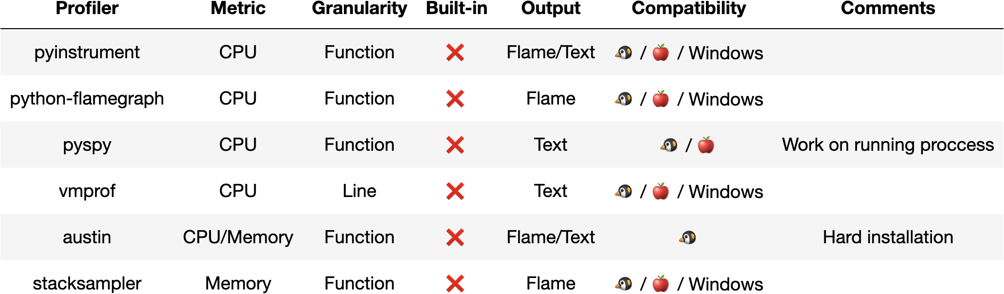
I am going to only cover pyinstrument, which measures the process CPU by sampling and recording statistics every one millisecond. It not built-in for Python, so installation is required, and it does not come with IPython magic.

a table of performance statistics for the sentence_correction function of pyinstrument — We can see our sentence_correction function took 0.28 seconds. All of it spent on the candidate function, and when we drill down the edits1 takes 0.1 seconds (40%). We can see that we have much less function (and noise) in the hierarchy thanks to the statistical nature of pyinstrument.

There are many more online profilers out, and the online profiling landscape ️️️️looks as follows:

table comparing several online profiling tools — The online profiling landscape ️️️️

‍

Online profilers have the following pros and cons

They allow us to pinpoint the bottlenecks.
They are not deterministic.
Still, they introduce overhead (marginal).
They are really easy to use.
They can’t tell us which inputs are slow.

We covered a lot of tools in this article. Now you have the ability to find the bottlenecks in 99% of the use cases.

‍

The Last Percent

But we still can’t tell which inputs will slow our program, and we have a problem if we want to profile an exotic metric like the number of context switches.

If by any chance you did not find any profiler to fit your problem,
you can create your own profiler:

You can create a custom offline profiler by using either cProfile or sys.settrace and sys.setprofile.
You can create a custom online profiler by using either setitimer or ptrace.
You can attach Python code to a running process using pyrasite.

To mitigate the fact profilers can’t tell us which inputs are slow, we can use logging in conjunction with profiling. Logging allows us to record whatever we want, without a performance penalty. But you need to add logging upfront or you are out of luck.

Pro Tip: Record hot function inputs and duration.

We found the bottleneck, now what? We simply need to fix the problem — easier said than done. Then we must watch for performance regressions. Optimized code tends to be a candidate for refactoring. We need to make sure we don’t reintroduce the same issues again.

‍

Last Words

In this article, we began by explaining why we should care about performance and finding our bottlenecks. Next, we walked through how we can use profilers to find those bottlenecks and make our users happy.

I hope I was able to share my enthusiasm for this fascinating topic and that you find it useful. As always, I am open to any kind of constructive feedback.

Eli Trabelsi